ggstackplot examples

library(dplyr)
library(ggplot2)
library(ggstackplot)

Example 1: high altitude balloon flight

Load example data

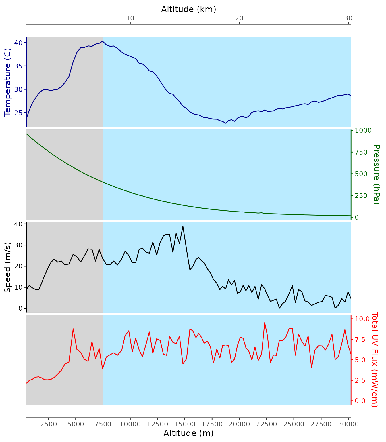
The data in this example are from measurements acquired on a scientific high altitude balloon flight. Caro, T.A., Wendeln, M., Freeland, M. et al. Ultraviolet light measurements (280–400 nm) acquired from stratospheric balloon flight to assess influence on bioaerosols. Aerobiologia 35, 771–776 (2019). https://doi.org/10.1007/s10453-019-09597-9

hab_data <- readRDS("HAB_example_data.RDS") |>
  slice_head(n = 100)

head(hab_data)
#> # A tibble: 6 × 5
#>   `Temperature (C)` `Pressure (hPa)` `alt (m)` speed `Total UV Flux (mW/cm)`
#>               <dbl>            <dbl>     <dbl> <dbl>                   <dbl>
#> 1              23.7             961.      480.  8.94                    2.13
#> 2              25.5             932.      744. 10.9                     2.47
#> 3              27.0             903.     1006   9.77                    2.61
#> 4              28.2             869.     1327.  8.90                    2.88
#> 5              29.1             841.     1612.  8.74                    2.92
#> 6              29.7             815.     1889. 12.2                     2.78

Visualize example data

hab_data |> 
  ggstackplot(
    x = `alt (m)`,
    y = c(`Temperature (C)`, `Pressure (hPa)`, `Speed (m/s)` = `speed`, `Total UV Flux (mW/cm)`),
    color = c("darkblue", "darkgreen", "black", "red"),
    alternate_axes = TRUE,
    switch_axes = TRUE,
    shared_axis_size = 0.3,
    overlap = 0.1,
    template =
      ggplot() +
      scale_x_continuous(
        name = "Altitude (m)",
        n.breaks = 12,
        sec.axis = sec_axis(
          name = "Altitude (km)",
          trans = ~ . / 1000
        ),
        expand = c(0, 0)
      ) +
      expand_limits(x = 0) +
      geom_rect(ymin = -Inf, ymax = Inf,
                xmin = 0, xmax = 7500,
                fill = "lightgray", color = NA,
                alpha = 0.1) +
      geom_rect(ymin = -Inf, ymax = Inf,
                xmin = 7500, xmax = 35000,
                fill = "lightblue1", color = NA,
                alpha = 0.1) +
      theme_stackplot(),
    add = list(
      `Temperature (C)` = geom_path(),
      `Pressure (hPa)` = 
        geom_path() +
        theme(axis.text.x = element_text(angle = 45, hjust = 0)),
      `Speed (m/s)` = geom_path(),
      `Total UV Flux (mW/cm)` = 
        scale_y_continuous(limits = c(0, 10), sec.axis = dup_axis()) +
        geom_path() 
    )
  )
#> Scale for y is already present.
#> Adding another scale for y, which will replace the existing scale.